
Image: Jonathan Knowles via Getty Images.
If you regularly use Microsoft Excel to create spreadsheets with many rows and columns, you know that finding information can be complicated, especially when you need to match information presented in one of the first rows of the table. . and another on line 150 for example.
To do this, you can simply freeze the first rows, so that their data remains visible when you scroll through the rest of the sheet. So, you can use any row or column as a legend or header for your spreadsheet, then freeze it for use with a remote part of the same spreadsheet.
The following demonstration is carried out in the Microsoft Excel software. If you are using similar software from another publisher (Google Sheets, LibreOffice Calc), the functionality may be presented slightly differently.
How to freeze rows in Excel?
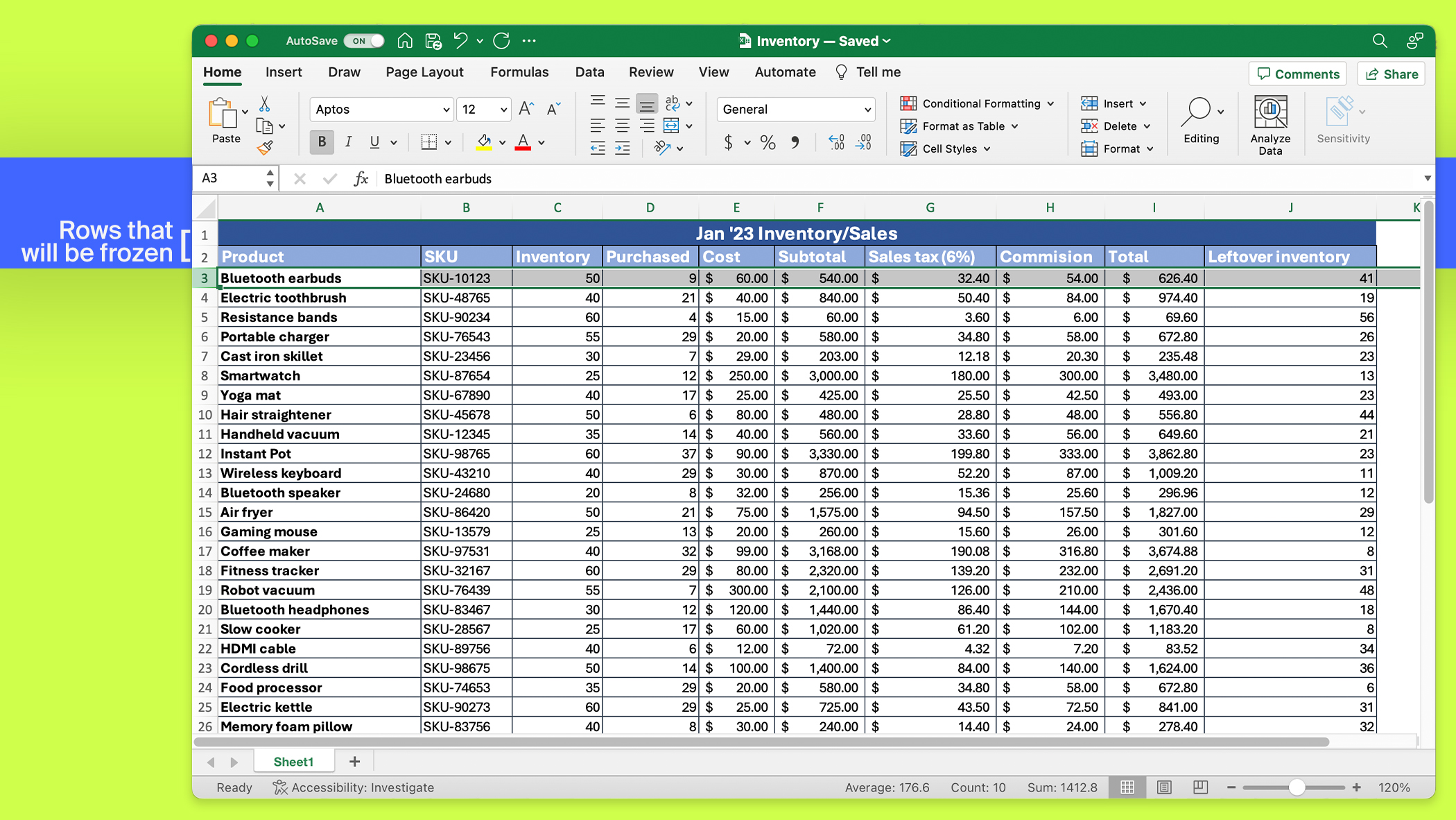
1. Select the line below the one you want to freeze
If the row you want to freeze is row 3, select row 4. The row above the one you select is the one that will be frozen.
In the example below, the header of my table is on lines 1 and 2, and the quantifiable data starts on line 3. I need to freeze lines 1 and 2 to find my way around , so I select line 3.
Screenshot by Maria Diaz/ZDNET.
2. Freeze the desired lines
Once you have selected the row below the one(s) you want to freeze, go to the tab Displaythen click Freeze Panes > Freeze Panes.
You can now freely scroll the rows and columns of the spreadsheet: frozen cells remain visible regardless.

Screenshot by Maria Diaz/ZDNET.
How to freeze columns in Excel?
Excel may automatically freeze the first column of a worksheet if you go to View > Freeze Panes and you select Freeze the first column.
If you want to freeze another column, select the one to its right then select View > Freeze Panes > Freeze Panes.
How to compare data by freezing cells?
Freezing rows or columns can help you compare data in several different places in a spreadsheet.
For example, to compare line 12 and line 87, select line 13 and click Freeze the shutters. Line 12 will therefore remain frozen when you scroll to line 87, making it easy to compare the data contained in the two lines.
How to unblock rows or columns in Excel?
So that your rows and/or columns are no longer frozen, simply return to View > Freeze Panes and select Release the shutters.
Source: ZDNet.com