Formulas and functions are the most powerful tool in Excel. You can even perform complex calculations in no time with functions in Excel.
Enlarge
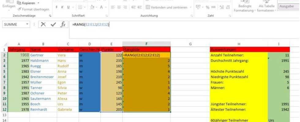
Evaluation with Excel formulas. The matrix formula that we will introduce to you in the course of this article is currently being used here.
© 2014
The Microsoft Excel 2016 spreadsheet offered over 400 functions – from simple arithmetic tasks such as addition (SUM function) to complex evaluations of the data in which values are compared (INDEX function). Microsoft presents all available functions on this website. This makes it easy to deal with complex data sets – but only if you know how formulas and functions work in Excel.
The functions presented here can not only be used with Excel 2013 or Excel 2016, but also work with older versions of Excel. The functions presented here also correspond to the functions in Excel 2011 for Macintosh.
You have to try whether the formulas presented here also work in the current Excel version 2019. The likelihood of this, however, is great.
The main innovation of Excel 2016 compared to the previous version 2013 was above all the extended visualization functions. This guide explains how Office 2016 works specifically on the Mac. Almost all functions of the previous Windows version, Excel 2013, are now also available on the Macintosh.

Enlarge
Excel shows you all available functions here.
You can display all functions available in Excel by selecting the “Formulas” tab and then clicking the “Insert function” button. In the window that then opens, select “All” under “Select category”. Then Excel shows all available functions in the selection window below. With a click of the mouse you get a short description of each function.
Formulas: The basis of functions in Excel
Before we get to the Excel functions like VLOOKUP or matrix formulas, let’s first explain their basis: the formulas.
You always write the formula in the formula bar and it always begins with an equal sign (=). A simple example: Let Excel calculate the result of the sum 113 + 253. To do this, click on any cell, write = 113 + 253 in the formula bar and press the Enter key. The result of the total – 366 – is immediately displayed in the previously clicked (“activated”) cell.

Enlarge
Simple example of a formula. A click on the symbol ƒx offers help on the typed formula
© 2014
Most of the time, however, you are calculating with values that are already in the table. You don’t enter numbers, just describe where they are entered. To do this, use the Excel coordinate system: Rows are numbered according to the scheme 1, 2, 3, etc., columns are displayed alphabetically with A, B, C, etc. The cell at the top left is A1, the one to the right is B1 and the one below is A2, etc.

In the screenshot above, cell A1 contains the number 113 and A2 253. For the calculation, Excel refers to cells, so the coordinates A1 and A2 of the cells are called “reference”. The formula that we enter for cell A3 is = A1 + A2. The displayed result in A3 is again 366.
Conditional formatting

With the “Conditional Formatting” in the Excel start menu, you can specify rules and values on the basis of which Excel will design your table. For example, enter 50 for “Less than” and select “Light red filling 2”, then Excel will store all values in the table that are smaller than 50 in light red.
If you later change values in the table, you will see that the results of your formulas also adapt immediately. This allows you to keep track of complex tables with many values. The same applies to tables that are constantly updated. You no longer use Excel only as a data storage device, but as a complex evaluation program for your data.
Relative and absolute cell references

© Vierfarben Verlag
By default, Excel automatically adapts cell addresses when they are filled out in rows and columns (relative cell references). If you want to avoid this and insert fixed, absolute cell references, you have to insert a dollar sign in the name of the desired cell.
Functions in Excel
With this type of formula use, Excel would not be able to make really complex calculations possible. That is why the software goes one step further and offers the so-called functions. An example: Instead of writing = A1 + A2 in the example above, we simply tell Excel what we want to do: We need the sum. Excel provides the SUM function of the same name for adding.
Video course “Excel Formulas & Functions & Pivot Tables Masterclass!” at Udemy

Enlarge
The result of = SUM (A1: A2 can be seen on the screenshot on the right.
A function consists of the capitalized name, followed by individual cells or an entire cell range in brackets () as well as other parameters – each with; separated. For a cell range, enter the coordinates of the first and last cells to be taken into account, separated by a colon. The formula for the example is = SUM (A1: A2), but it could also be = SUM (A1: A23) or = SUM (A: A) if the entire column A is to be added. Without a function, the total would be more difficult to calculate. The easiest way to enter cell ranges is to mark the cells with the mouse when entering the formula instead of typing in the cell references.
Book tip: Excel 2016. The instructions in pictures

The book Excel 2016 was published by Vierfarben-Verlag, which belongs to Rheinwerk Verlag GmbH (formerly Galileo Press). The instructions in pictures for 9.90 euros in the series “See how it’s done”. On around 360 pages, the two authors offer a comprehensive overview of Excel 2016 in all its facets. The specialty of this book: It is a picture-by-picture instruction, every function described in the book is presented with a screenshot. The corresponding explanations are right next to the screenshot. This approach is particularly suitable for readers who value consistent and meaningful illustrations and who do not want to read excessively long passages of text. This book is also very suitable for Excel beginners. The authors deal with the complex subject of “formulas and functions” on 73 pages, which means that they are thoroughly comprehensive.
Notice:
All functions can be found under the Formulas tab. The function libraries there are sorted by groups.
Function assistant

You can use the function wizard to search for a suitable function. To do this, click on the Formula tab on the fx icon (insert function) on the far left in the menu ribbon. A small window called “Insert function” opens. Enter your search term in the input field under “Search for a function”, in our example it is “Link texts”. Then click OK”. And Excel will show you suitable functions.
On the next page we explain “Complex Functions”.
More tips, tricks and tools for everything to do with Excel:
The 5 most important Excel macros for everyday life
Three smart Excel tools and one alternative to Excel
Ten Excel Tips for Office Professionals
Create pivot tables in Excel – this is how it works
The ten best Excel functions
In just 8 steps to the perfect Excel spreadsheet
The 5 most important Excel macros for everyday life
Calculating with Excel – formulas and functions